An Introduction To Bayesian Optimization from a Performance Engineering Perspective
Introduction
In this post, I go over details of the Bayesian Optimization algorithm in a language and implementation agnostic way to highlight what it is and what are the advantages and disadvantages of using it in the context of performance engineering. Subsequently, I go over the components of this algorithm and highlight some implementation details and finally present some implemented examples.
The format of this post is done in a Socratic way or in the form of pertinent questions and answers rather than presenting topics; I found that this was the best way I understood the mechanics of this algorithm and all its associated details.
It's worth noting this blogpost is based off a submission I made to an annual event called "FSharp Advent", the full post of which can be found here.
Motivation
The motivation behind this post is 2-fold:
- I have been very eagerly trying to learn about Bayesian Optimization and figured this was a perfect time to dedicate myself to fully understanding the internals by implementing the algorithm.
- I am yet to find a library (if you know of one, please let me know) that naturally combines Bayesian Optimization with Performance Engineering in .NET to come up with optimal parameters to use for a specified workload.
What is Bayesian Optimization?
Bayesian Optimization is an iterative optimization algorithm used to find the most optimal or best element vis-à-vis some criterion known as the objective function from a number of alternatives. The best element is known as the global optima and can be either the one that minimizes or maximizes the said criterion.
An examples of the setup of optimization methods are:
- Finding the number threads needed to maximize the throughput for a particular workload.
- Finding the right memory limit to set on a container so that we have the lowest memory consumed if we are on a tight memory budget.
- Finding the most aggressive parameters that maximize the CPU usage and thereby maximize the throughput.
Why Use Bayesian Optimization?
Where Bayesian Optimization shines in comparison to other optimization methods is when the criteria to be optimized, more formally known as the Objective Function is a black box.
A black box function indicates that there is a lack of mathematical form of the objective function or other known mathematical properties that allow us to use numerical techniques to solve for the optimal value.
Examples of black box functions include:
- Garbage Collection based Pause Duration for a particular workload.
- The number of CPU cycles taken to compute the digits of PI up to 100 decimal points.
- Where and how to drill to get the most optimum amount oil extracted at an oil well.
These black box functions are fairly common in the world of performance engineering where the objective functions are noisy are unknown as factors such as machine state or the non-deterministic behavior the OS scheduler effects the overall performance of a process.
The following table summarizes the comparison of 2 other popular optimization methods:
| Optimization Method | What it is? | Disadvantages |
|---|---|---|
| Grid Search Optimization | Grid Search Optimization entails exhaustively searching through a manually specified subset of parameters for which the objective function is to be calculated for. | Grid search can be unfeasible because its often computationally impossible to compute the objective function over all possible specified values as computing these objective functions can be expensive. |
| Random Search Optimization | Random Search Optimization entails picking random inputs to compute | Since we are picking inputs randomly, there could be high chance we don't choose the optima. |
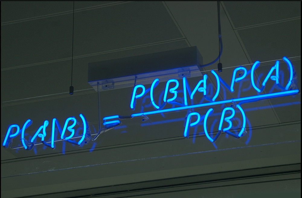
What is Bayesian About The Bayesian Optimization Algorithm?
The efficiency of the Bayesian Optimization Algorithm stems from the use of the Bayes Theorem to choose where to search next for the global optima based on information in the past. In other words, we are incorporating knowledge about the objective function and places where we have the optimum values with each iteration.
For those who are interested, a primer of the Bayes Theorem can be found here.
What are Some Disadvantages of the Bayesian Optimization Algorithm?
- Results Are Extremely Sensitive To Model Parameters: Having some prior knowledge of the shape of the objective function is helpful as otherwise, choosing the wrong parameters results in a need for a higher number of iterations or sometimes convergence to the optima isn't even possible. Finding the right model parameters can take effort as it requires experimentation.
- Model Estimation Takes Time: Since the objective function or the criterion we are trying to optimize is a black box, getting to a point where we have a reasonable proxy of it can take quite a few iterations especially if the objective function isn't a simple curve.
What are the Components of the Bayesian Optimization Algorithm?
There are 3 main components of this algorithm:
- A Proxy of the Objective Function or the Surrogate Model: The surrogate model serves as our proxy of the objective function.
- The Function That Helps Decide Where to Search Next or the Acquisition Function: The acquisition function helps the algorithm to discern where to search next in the search space.
- The Iteration Loop: The loop facilitates iterating over data points that update the proxy of the objective function and choose where to search next so as to get to the global optima.
Diagrammatically, this looks like:
To be more specific, based on some range of generated inputs, we are iterating over each of these points to update our proxy of the objective function and choosing where to search next so as to best get to the most optimum value.
Examples
I have added the following experiments that'll help explaining the implementation, setup and results in F#. Before diving in I thought I'd cover how do interpret the charts from the results below.
An example of a chart looks like the following:
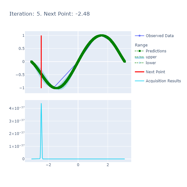
- Predictions: The predictions represent the mean of the results obtained from the underlying model that's the approximate of the unknown objective function. This model is also known as the Surrogate Model and more details about this can be found here. The blue ranges indicate the area between the upper and lower limits based on the confidence generated by the posterior.
- Acquisition Results series represents the acquisition function whose maxima indicates where it is best to search. More details on how the next point to search is discerned can be found here.
- Next Point: The next point is derived from the maximization of the acquisition function and points to where we should sample next.
- Observed Data: The observed data is the data collected from iteratively maximizing the acquisition function. As the number of observed data points increases with increased iterations, the expectation is that the predictions and observed data points converge if the model parameters are set correctly.
1. Computing the Maximum Value of the Sin function between π and -π
Sin(x) is a Trigonometric Function whose maximum value is 1 if the input is π/2 when the range is between −π and π. Since we know the analytical form of the function, this simple experiment can highlight the correctness of the algorithm (within an acceptable margin of error). A Polyglot notebook of this experiment can be found here.
The experiment can be setup in the following way making use of the library I developed that implements the Bayesian Optimization algorithm based on the library I created:
open Optimization.Domain
open Optimization.Model
open Optimization.Charting

let iterations : int = 10
let resolution : int = 20_000

// Creating the Model.
let gaussianModelForSin() : GaussianModel =
    let squaredExponentialKernelParameters : SquaredExponentialKernelParameters = { LengthScale = 1.; Variance = 1. }
    let gaussianProcess : GaussianProcess =  createProcessWithSquaredExponentialKernel squaredExponentialKernelParameters
    let sinObjectiveFunction : ObjectiveFunction = QueryContinuousFunction Trig.Sin
    createModel gaussianProcess sinObjectiveFunction ExpectedImprovement -Math.PI Math.PI resolution

// Using the Model to generate the optimaResults.
let model         : GaussianModel = gaussianModelForSin()
let optimaResults : OptimaResults = findOptima { Model = model; Goal = Goal.Max; Iterations = iterations }
printfn "Optima: Sin(x) is maximized when x = %A at %A" optimaResults.Optima.X optimaResults.Optima.Y
The results are:
The function is smooth and therefore, the length scale and variance of 1. respectively are sufficient to get us to a good point where we achieve the optima in a few number of iterations. The caveat here, however, was the selection of the resolution that had to be high since we want a certain degree of precision in terms of calculating the optima.
This experiment is an example of a mathematical function being optimized. More examples of these can be found here in the Unit Tests.
Experiment 2: Minimizing The Wall Clock Time of A Simple Command Line App
The Objective Function meant to be minimized here is the wall clock time from running a C# program, our workload, that sleeps for a hard-coded amount of time based on a given input. The full code is available here.
The gist of the trivial algorithm is the following where we sleep for the shortest amount of time if the input is between 1 and 1.5, a slightly shorter amount of time if the input is >= 1.5 but < 2.0 and the most amount of time in all other cases. The premise here is to try and see if we are able to get the optimization algorithm detect the inputs that trigger the lowest amount of sleep time and thereby, the minima of the wall clock time of the program in a somewhat deterministic fashion.
The results are:

The result was: Optima: Simple Workload Time is minimized when the input is 1.372745491 at 0.13 seconds. This was a success as we force the main thread to sleep in the interval [1., 1.5) and the input: 1.37274591 is in that range!
The inputs here didn't require a highly precise resolution as the previous experiment and therefore, I set them to a moderately high amount of 500. I had to play around with the number of iterations as this was a more complex objective function in the eyes of the surrogate model; my strategy here was to start high and make my way to an acceptable amount. The other parameters i.e. Length Scale and Variance were the same, as before.
Experiment 3: Minimizing the Garbage Collection (GC) Pause Time % By Varying The Number of Heaps
The workload code, that can be found here, first launches a separate process that induces a state of high memory; the source code for the high memory load inducer can be found here. Subsequently, a large number of allocations are intermittently made. While this workload is executing, we will have been taking a ETW Trace that'll contain the GC Pause Time %. The idea behind the experiment is to stress the memory of a machine and see how bursty allocations perform with varying Garbage Collection heaps the value of which, is controlled by 2 environment variables: COMPlus_GCHeapCount and COMPlus_GCServer where the former needs to be specified in Hexadecimal format indicating the number of heaps to be used bounded by the number of logical processors and the latter is a boolean (0 or 1).
The result of this experiment is: Optima: GC Pause Time Percentage is minimized when the input is 12.0 at 2.51148003.

To double check we are actually achieving the minima, I conducted a grid search and corroborated the values and the result were:
Optima: GC Pause Time Percentage is minimized when the input is 12.0 at 2.247975719.
| Heap Count | Percentage Pause Time In GC |
|---|---|
| "1" | 4.7886298 |
| "2" | 4.236894341 |
| "3" | 4.71068455 |
| "4" | 3.870396061 |
| "5" | 4.460504767 |
| "6" | 3.473897596 |
| "7" | 3.276429007 |
| "8" | 3.203552845 |
| "9" | 2.846175963 |
| "10" | 2.563527965 |
| "11" | 2.434899728 |
| "12" | 2.247975719 <- MIN |
| "13" | 2.536508289 |
| "14" | 2.528864583 |
| "15" | 2.400874153 |
| "16" | 2.362189349 |
| "17" | 3.375737401 |
| "18" | 5.864851149 |
| "19" | 5.352540323 |
| "20" | 6.907995823 |
Conclusion
If I had to encapsulate the takeaways from this post into 3 main lessons, these would be:
- Bayesian Optimization algorithm, an iterative optimization algorithm used to find the most optimal or best element vis-à-vis some criterion known as the objective function from a number of alternatives.
- Bayesian Optimization is an effective technique when the objective function or the criterion to consider is a black-box.
- The disadvantages of Bayesian Optimization are that it is extremely dependent on the input parameters and can be slow.